How Do State Space Models Work in Modern AI? S4 to Mamba

I still remember the exact moment a long document blew through my transformer's attention memory budget on a mid-size GPU, and the job died with a CUDA out-of-memory error at 2am with nobody around to page. That week I went looking for something that didn't scale quadratically with sequence length, and that's how I ended up staring at state space models until the equations finally clicked. If you've ever wondered how do state space models work under the hood, the honest answer is: they don't attend to anything.

Instead they carry a compact hidden state forward, token by token, updating it the way a running average updates - except the update rule is learned, structured, and in newer variants like Mamba, selective about what it keeps.

That distinction - fixed dynamics versus input-dependent dynamics - is the whole story of how this field went from a control-theory curiosity to a serious LLM architecture. This piece walks through the actual math, one input at a time, from the continuous equations to the discrete recurrence to the parallel scan that makes it fast on real hardware.

How State Space Models Work: State, Input, and Output

At its core, a state space model in AI is a sequence layer that keeps a small, fixed-size latent state instead of storing every past token explicitly. Think of it like a running memory tape you update with each new word, rather than a growing list you re-read every step. That single design choice is why state space models are used at all: the compute per step stays constant, the inference footprint doesn't balloon with context length, and the model can still carry long-range signal without rereading history.

Picture reading a novel and only keeping a mental summary of the plot so far - that summary is your hidden state, the current sentence is your input, and whatever you say aloud about the story is the output.

The State and Output Equations

Formally, this is two equations: h′(t) = Ah(t) + Bx(t), and y(t) = Ch(t) + Dx(t).

Each matrix plays one role:

• A governs how the existing state evolves on its own, with no input at all.
• B decides how much of the current input gets injected into that state.
• C reads the state back out into an output.
• D is an optional shortcut straight from input to output.

Unlike an attention map, there's no per-token weight you can point at and say "that's why it remembered this." I've spent time staring at trained A and C matrices looking for something interpretable and never found much - the hidden state is a learned compressed memory, not a lookup table.

From Continuous Dynamics to a Discrete Sequence Layer

Those two continuous equations describe a signal flowing smoothly through time, but tokens don't arrive smoothly - they arrive one at a time, discretely. Before A and B can process a token stream, they need to be converted into discrete-time versions, Ā and B̄, that step forward once per token instead of continuously.

That conversion happens through a step size Δ, which represents how much "time" one token or sample is worth. It's fed through a zero-order hold, which assumes the input stays constant across that tiny interval, letting you integrate the continuous equation exactly and get closed-form Ā and B̄ from A, B, and Δ.

Once you have those, the model runs as a plain recurrence: h_k = Āh_{k-1} + B̄x_k, and y_k = Ch_k + Dx_k. No integrals left - just matrix multiplies at each step, which is why this shape can slot into a training loop like an RNN, and why the same layer can handle irregularly sampled data by simply varying Δ per step.

Three Equivalent Views: Recurrence, Convolution, and Scan

The recurrence h_k = Āh_{k-1} + B̄x_k is the same linear system as a convolution - you're just choosing where to do the algebra. Unroll it far enough and every output becomes a weighted sum of past inputs: y_k = CB̄x_k + CĀB̄x_{k-1} + CĀ²B̄x_{k-2} + …

That sequence of terms - CB̄, CĀB̄, CĀ²B̄, and so on - is the SSM kernel, and convolving it against the input sequence gives you identical outputs to running the recurrence step by step. Same math, different shape.

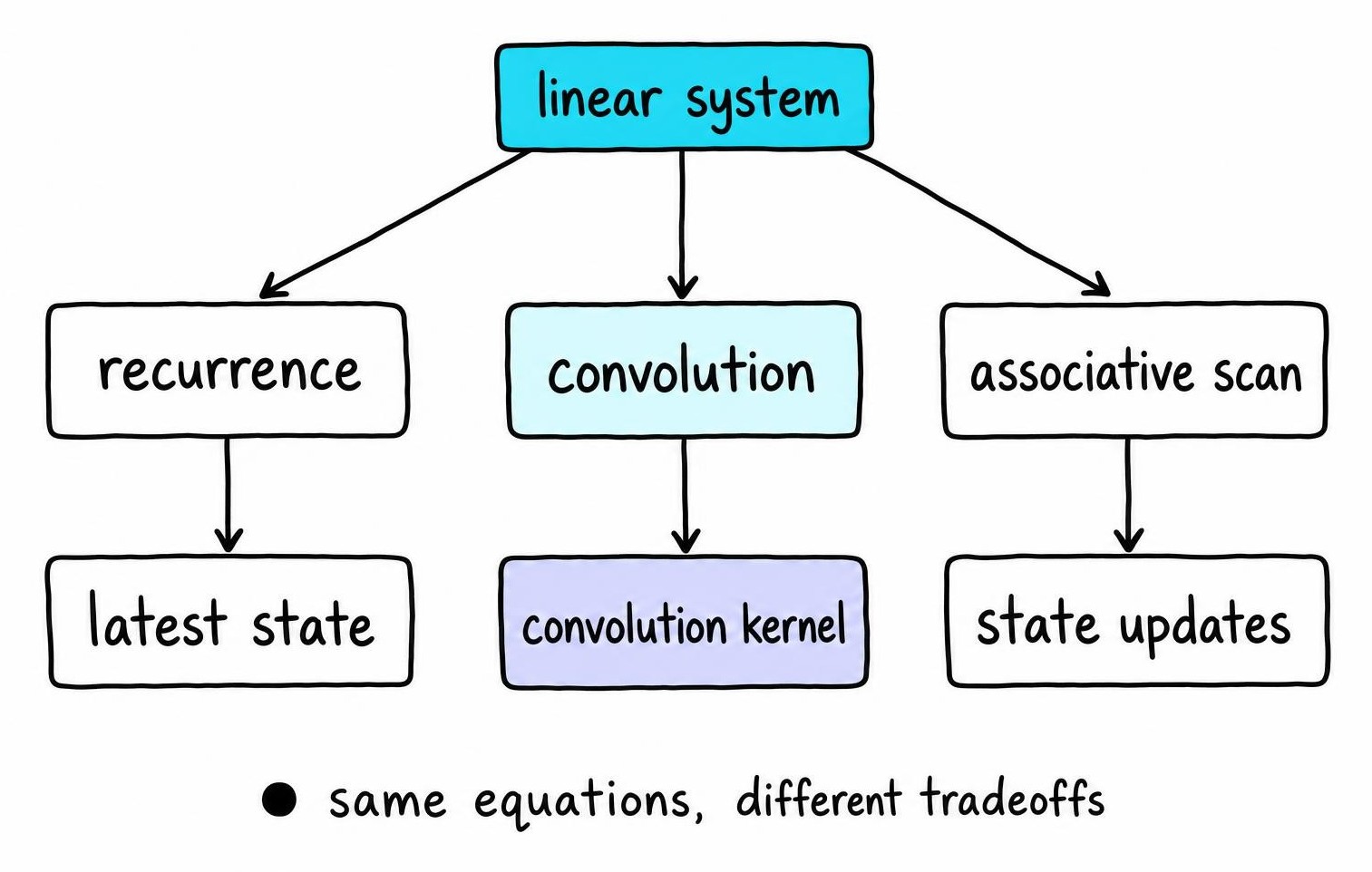
There's a third view worth knowing: the associative scan. Because the state update is a linear, associative operation, you can compute chunks of the sequence in parallel and combine them afterward, instead of forcing a strictly sequential loop. This is what lets modern selective SSMs stay fast on GPUs without giving up the recurrent formulation entirely.

When Each Representation Is Useful

• Training on full sequences: precompute the convolution kernel or run a parallel scan - both exploit hardware parallelism across the whole batch.
• Autoregressive generation: fall back to the plain recurrence, since only the last hidden state needs to survive between steps, not the whole kernel.

I once inherited a generation loop that rebuilt and reconvolved the entire SSM kernel on every new token instead of carrying the last hidden state forward. The code looked fine and tests passed, but latency crept up with every token generated instead of staying flat. Picking the wrong representation for the job is the single most common inefficiency I see in half-built SSM code.

Structured State Space Models: How S4 Learns Long Memory

Here's the problem I ran into first: if A is just a dense matrix you let gradient descent optimize freely, training gets ugly fast. A dense N×N matrix costs O(N²) per step, and nothing stops its eigenvalues from drifting past 1, so the hidden state explodes or the gradient vanishes over long sequences.

S4 fixes this by constraining A's structure up front instead of leaving it fully free. It uses a specific normal-plus-low-rank form that lets the long convolution kernel be computed far more cheaply than a naive dense recurrence would allow [1].

The initialization behind that structure is HiPPO, a construction designed to compress a signal's entire history into a fixed-size state without discarding older information the way a naive exponential decay would [2]. It's not a heuristic bolted on after the fact; it's derived so the state approximates past inputs under a chosen basis. S4's initialization is designed to retain older signal that a naive decay discards, which is the mechanism behind its long-range dependency results.

The pipeline, then: structured continuous A and B, HiPPO-based initialization, discretization into Ā/B̄, and a trainable convolutional or recurrent layer sitting on top.

Why the Transition Matrix A Matters

A's eigenvalues set the physics of memory. Eigenvalues near the unit circle decay slowly - long memory - while ones further inside decay fast, and any imaginary component introduces oscillation rather than plain fade.

Different dimensions of the same state can hold different eigenvalues simultaneously, so one channel tracks a fast local pattern while another tracks something spanning thousands of tokens. That's structure the architecture provides; gradient descent then only tunes parameters within that stable envelope, rather than rediscovering stability from scratch - a distinction worth keeping in mind if you're comparing these layers to transformers in a head-to-head technical breakdown.

Selective State Space Models and Mamba's Core Mechanism

S4's structured A buys speed, but it buys it by keeping Ā, B̄, and C fixed for every token - the update rule for word 3 is identical to the update rule for word 3,000. That's fine for smooth signals, useless for language, where the right thing to remember depends entirely on content: a name matters, a filler word doesn't.

Mamba's fix is to stop treating Δ, B, and C as learned constants and make them functions of the current input instead. Each token now projects its own step size and injection/readout vectors, so the layer can dilate Δ to skim irrelevant text or shrink it to lock onto something worth keeping.

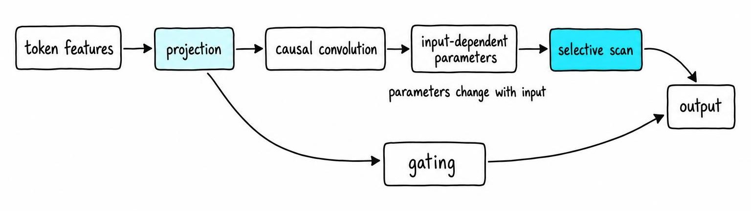
Selection isn't a separate attention-like lookup bolted onto the SSM - it's baked into the same state-update parameters, just made input-dependent. A Mamba block wraps this in a fairly plain shell: input projection, a short causal convolution for local context, a gating branch, the selective SSM scan itself, then an output projection. For a deeper visual walkthrough of these blocks, this visual guide to Mamba is worth the read.

How the Hardware-Aware Selective Scan Runs

Because Ā/B̄ now change every step, you lose the single global convolution kernel S4 relied on - there's no fixed kernel to precompute when the rule shifts token to token. The scan has to run as a genuine recurrence, computed in parallel chunks and fused into custom GPU kernels with selective recomputation, since materializing every intermediate state in slow memory would be too costly. Linear time in sequence length is a math fact; realized wall-clock speed depends entirely on how tightly that scan is fused to hardware.

Training, Fine-Tuning, and Debugging an SSM Layer

Before touching a training loop, map the shapes in your head:

• inputs: (B, L, D) - batch, sequence length, model dimension
• hidden state: (B, D_inner, N), where N is the per-channel state dimension
• selective parameters Δ, B, C: (B, L, D_inner) or (B, L, N) depending on which are made input-dependent

Get this wrong once and you'll pay for it quietly. I did exactly that on a side project: I'd transposed D_inner and N when writing the state update by hand, and the model trained fine on paper. Loss ticked downward every epoch, just noticeably slower than it should have. It plateaued early at a mediocre level, and nothing crashed - no shape error, nothing to grep for. I only caught it by writing a dumb, naive Python recurrence over a short 16-token sequence and comparing its output tensor to my "optimized" version step by step, at which point the mismatch on the very first state update jumped out immediately.

Training itself is unremarkable once shapes are right: gradients flow through the discretization step, through Δ's projection, through B/C's projections, and through the gating and output heads, all via ordinary backprop through the scan.

Fine-tuning a pretrained Mamba-style checkpoint works like fine-tuning any LLM - full-parameter updates for real capacity, LoRA-style adapters on the projection matrices when compute is tight, though adapter support here is less mature than for transformer stacks.

When something's off, check in this order:

• state values exploding or collapsing to zero over long sequences
• causal masking broken, letting future tokens leak into the scan
• Δ values pinned at initialization instead of varying per token
• padding tokens polluting the running state
• a naive Python recurrence disagreeing with your fused scan on short sequences - always test that first

State Space Models for LLMs and Machine Translation

SSMs show up in LLM work three ways: as full decoder-only backbones, as encoders paired with a different decoder, or as one layer type mixed into an otherwise ordinary transformer stack. That last hybrid pattern is the one I keep running into on real projects - a long-document summarization pipeline where swapping a chunk of attention blocks for selective SSM blocks cut memory pressure enough that I stopped babysitting sequence-length limits.

Machine translation results are genuinely mixed, and effectiveness depends heavily on training data volume, model scale, and whether the encoder gets full bidirectional context or only a causal pass over the source sentence. Long documents are where the efficiency argument actually earns its keep, since constant per-token cost avoids the attention blowup on long inputs. A fixed-size compressed state can still blur exact recall of a source token from ten sentences back, though, which matters when translation needs precise term consistency.

Practical Limitations of S4, Mamba, and Other SSMs

The fixed-size state is an information bottleneck by construction. It can't losslessly store arbitrarily long history, so tasks needing exact copying or precise retrieval of an early token - the same weakness that shows up in translation term consistency - often expose gaps transformers don't share, and there's no attention map to inspect when something goes wrong, just a compressed vector. Training stability needs care around Δ initialization and state scaling, selective SSMs add real implementation complexity on top of S4's already nontrivial machinery, and linear-time scaling is a property of the math, not a guarantee about your specific kernel, sequence length, or accelerator.

For a broader take on these tradeoffs against attention-based models, the state space model versus transformer comparison covers that ground directly, and IBM's overview of state space models is a solid plain-language reference too.

FAQ

How do state space models work?

They carry a fixed-size hidden state forward through a sequence, updating it at each step with a learned linear recurrence rather than attending back over every prior token. A continuous update rule, governed by matrices A, B, C, and D, gets discretized with a step size Δ so it can run token by token, and that same recurrence reshapes into a convolution or a parallel scan depending on whether you're training or generating.

What are state space models?

They're sequence layers, borrowed from control theory, that describe how a hidden state evolves given an input and how an output gets read back out of it. Modern variants like S4 and Mamba turn that into a trainable neural network layer.

What are state space models in AI?

In AI, they're an alternative to attention: constant compute per step, a compact latent state instead of a growing history, and variants like Mamba that make the update rule input-dependent so the layer learns what to keep and what to skip.

How effective are state space models for machine translation?

Results are mixed and depend heavily on scale, training data, and whether the encoder sees bidirectional context. They tend to shine on long documents where constant-cost processing avoids attention's blowup, but can lag on tasks needing exact recall of distant source tokens.

References

1. Kernel based low-rank sparse model for single image super-resolution - Jiahe Shi, Chun Qi (2018)
2. The Modified Airy Function Approximation Applied to the Double-Well Potential - N. Wine, J. Achtymichuk, F. Marsiglio (2025)